Stable operation of DC motor
During steady-state operation, The motor drives a load and speed will not vary at this stage. Constant speed means that there is no acceleration and $\frac{d\omega_m}{dt}=0$. Therefore:
$$T = J \frac{d \omega_m}{dt} + T_L $$
and hence, $T=T_L$, assuming the torque due to friction is zero for simplicity or that the load torque contains the useful load and friction values. To find out the operating point (Q), the operating point is defined by the intersection of the motor characteristic with the load characteristics. It means the motor will be running at the speed and the corresponding torque will be as shown in the figure below.
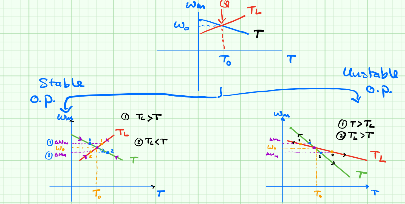
The condition for stable operation is $\frac{dT_L}{d\omega_m} \gt \frac{dT}{d\omega_m}$. Below is mathematical stability analysis proofing this condition.
$$T = T_L + J \frac{d\omega_m}{dt} \tag{a}\label{eq:a}$$
now in order to find out if the operting point Q in the figure above is stable, we perturb the torque by $\Delta T$ and monitor speed behaviour in small signal analysis sense.
$$\begin{align} T + \Delta T &= T_L + \Delta T_L + J \frac{d}{dt}(\omega_m + \Delta \omega_m) \tag{b}\label{eq:b}\\
\Delta T &= \Delta T_L + J \frac{d}{dt} \Delta \omega_m \tag{c} \label{eq:c}
\end{align}$$
Taking \eqref{eq:b} minus \eqref{eq:a} results in the small signal equation \eqref{eq:c}. Here we define of $\Delta T$ and $\Delta T_L$ are as follows:
$$\begin{align}\Delta T = \frac{dT}{d\omega_m} \cdot \Delta \omega_m \tag{d}\label{eq:d}\\
\Delta T_L = \frac{dT_L}{d\omega_m} \cdot \Delta \omega_m\tag{e}\label{eq:e}
\end{align}$$
substitution of \eqref{eq:d} and \eqref{eq:e} in \eqref{eq:c} yeilds
$$ \frac{dT}{d\omega_m} \cdot \Delta \omega_m = \frac{dT_L}{d\omega_m} \cdot \Delta \omega_m + J \frac{d}{dt} \Delta \omega_m \tag{f}\label{eq:f}$$
rearranging \eqref{eq:f} and solving for $\Delta \omega_m$
$$\begin{align}0 &= J \frac{d}{dt} \Delta \omega_m + \left [ \frac{dT}{d\omega_m} - \frac{dT_L}{d\omega_m} \right ] \tag{g}\label{eq:g}\\&\nonumber\\
\Delta\omega_m & = \Delta \skew{2}{\hat}\omega_m \cdot e^{-\frac{1}{J} \cdot \left [ \frac{dT}{d\omega_m} - \frac{dT_L}{d\omega_m} \right ]}\tag{h}\label{eq:h}\end{align}$$
where $\Delta\skew{2}{\hat}{\omega}_m$ is the initial condition of the motor speed.
$\Rightarrow$ if $t \rightarrow \infty$ then $\Delta\omega_m \rightarrow 0$ and accordingly $\left [ \frac{dT}{d\omega_m} - \frac{dT_L}{d\omega_m} \right ] \gt 0$ and the condition for steady-state is satisfied by \eqref{eq:i}
$$ \frac{dT_L}{d\omega_m} \gt \frac{dT}{d\omega_m} \tag{i}\label{eq:i}$$
Motoring and electric braking of Shunt/Sep. Excited DC motor
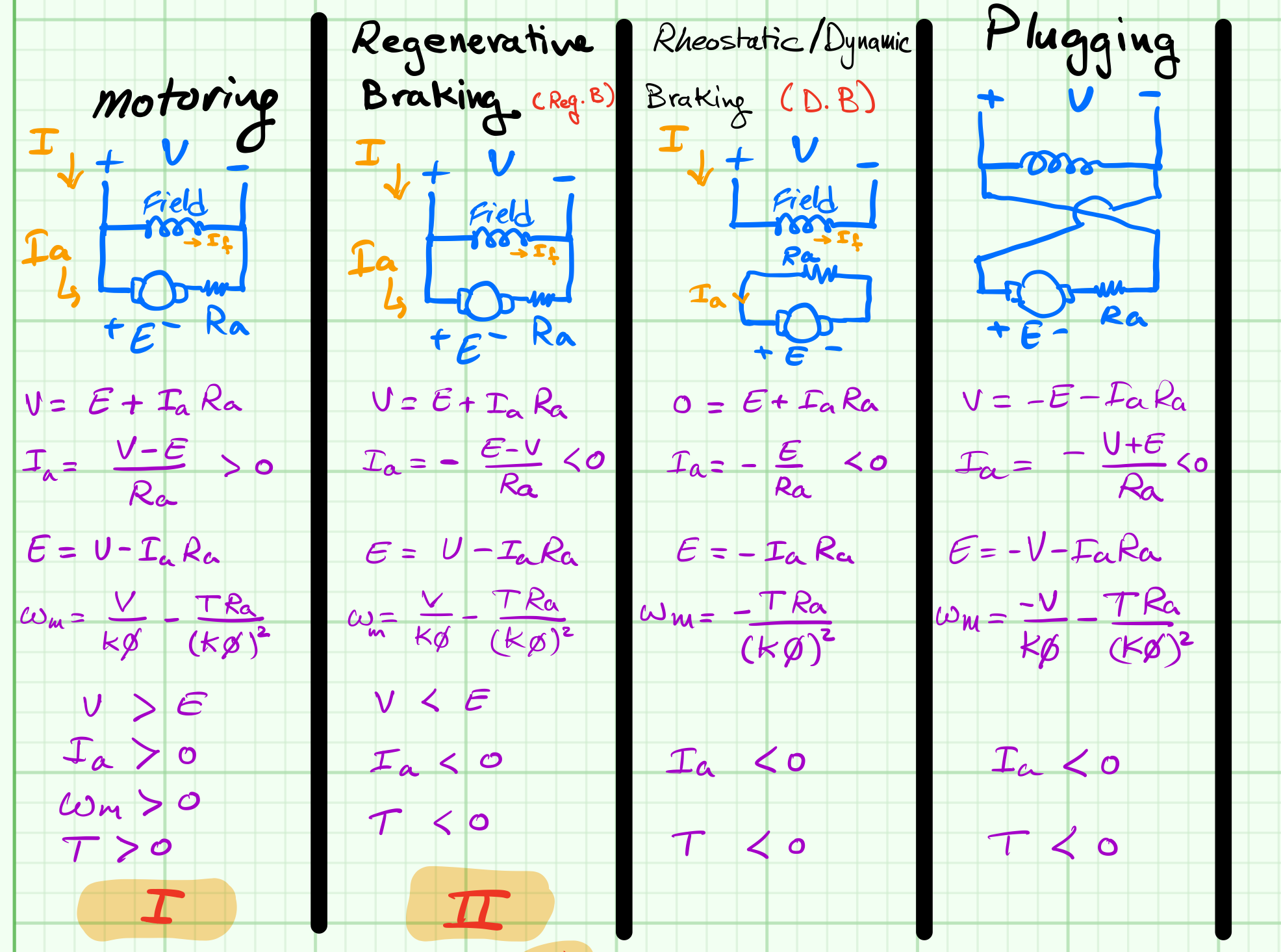
Motoring
$$V=E+I_a R_a\tag{1}$$
$$I_a=\frac{V-E}{R_a}\tag{2} \gt 0$$
$$E=V-I_a R_a\tag{3}$$
$$\omega_m=\frac{V}{K\phi}-\frac{T R_a}{(K\phi)^2}\tag{4}$$
Condition:
- $V\gt E$
- $I_a\gt 0$
- $T\gt 0$
- $\omega_m\gt 0$
Re-generative braking
$$V=E+I_a R_a\tag{5}$$
$$I_a=-\frac{E-V}{R_a} \lt 0\tag{6}$$
$$E=V-I_a R_a\tag{7}$$
$$\omega_m=\frac{V}{K\phi}-\frac{T R_a}{(K\phi)^2}\tag{8}$$
Condition:
- $V\lt E$
- $I_a\lt 0$
- $T\lt 0$
Dynamic/Rheostatic braking
$$0=E+I_a R_a\tag{9}$$
$$I_a=-\frac{E}{R_a}\lt 0\tag{10}$$
$$E=-I_a R_a\tag{3}$$
$$\omega_m=-\frac{T R_a}{(K\phi)^2}\tag{11}$$
Condition:
- $I_a\lt 0$
- $T\lt 0$
Plugging
$$V=-E-I_a R_a\tag{12}$$
$$I_a=-\frac{V+E}{R_a}\tag{13}\label{eq13}$$
$$E=-V-I_a R_a\tag{14}$$
$$\omega_m=-\frac{V}{K\phi}-\frac{T R_a}{(K\phi)^2}\tag{15}$$
Condition:
- $I_a\lt 0$
- $T\lt 0$
- eq.\eqref{eq13}: $R_a$ has to be sufficiently high to avoid high current damage
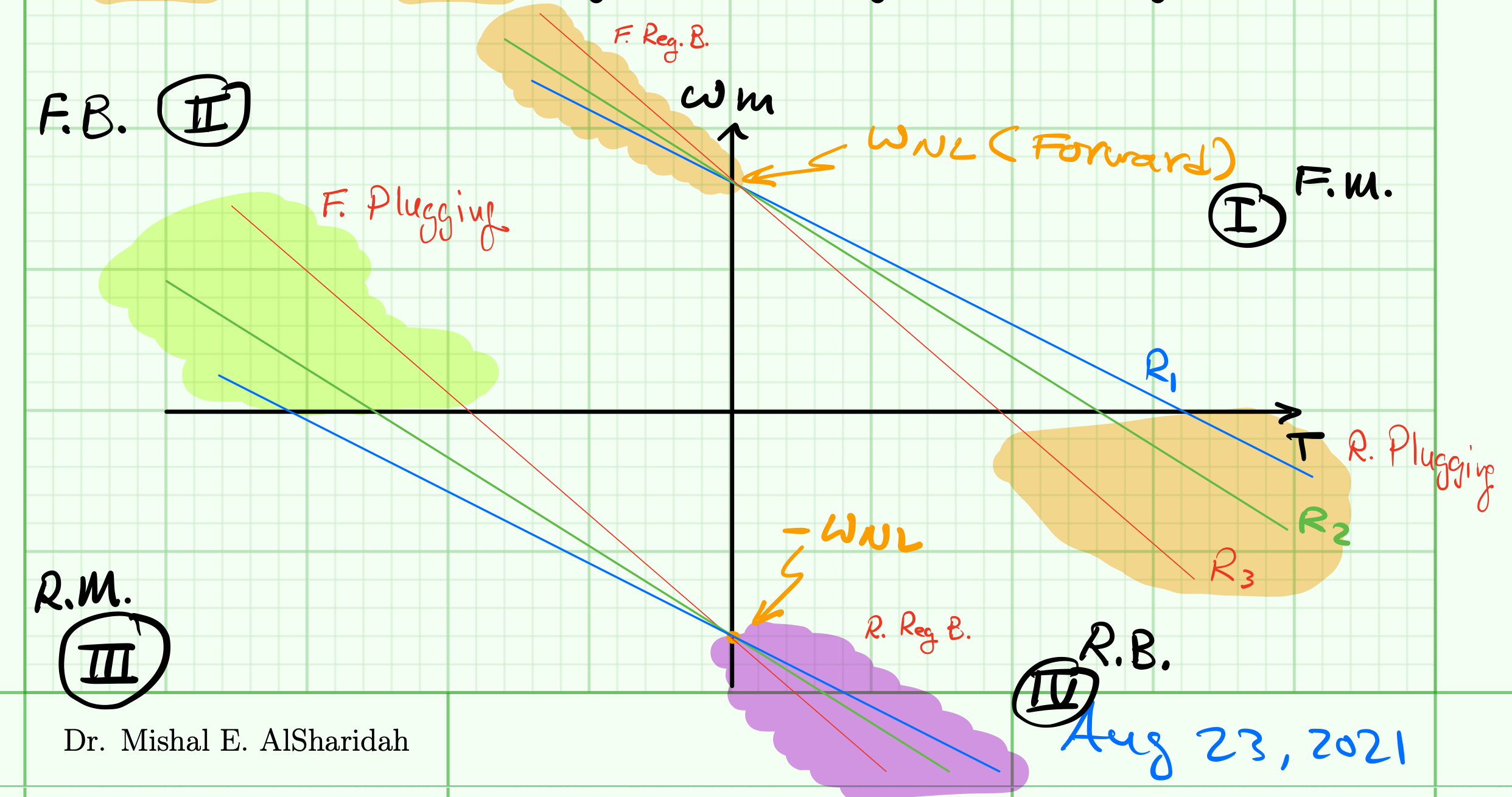
Summary of motoring and electrical braking of Shunt/Sep. excited DC motor
Quadrant operations